GEMM

Part 4 of How to make your models fast (LayerNorm | Introduction)

A worklog on making matrix multiplication fast in CUDA by fixing memory access, reusing tiles from shared memory, and computing multiple outputs per thread.

Authors

Affiliation

Anshuman Mishra

Independent researcher

Published

Sept. 18, 2026

The code for this chapter lives in kernels/gemm/.

We have already done GEMV, which was a matrix multiplied with a vector. GEMM is the same idea, except now we are multiplying a matrix with another matrix.

GEMM means GEneral Matrix-Matrix multiplication. Formally, we have

\[\mathbf{A}\in\mathbb{R}^{M\times K}, \qquad \mathbf{B}\in\mathbb{R}^{K\times N},\]

and our goal is to calculate

\[\mathbf{C}_{M\times N} =\mathbf{A}_{M\times K}\mathbf{B}_{K\times N}.\]

Every element of $\mathbf{C}$ is a dot product between one row of $\mathbf{A}$ and one column of $\mathbf{B}$:

\[C_{i,j}=\sum_{k=0}^{K-1}A_{i,k}B_{k,j}.\]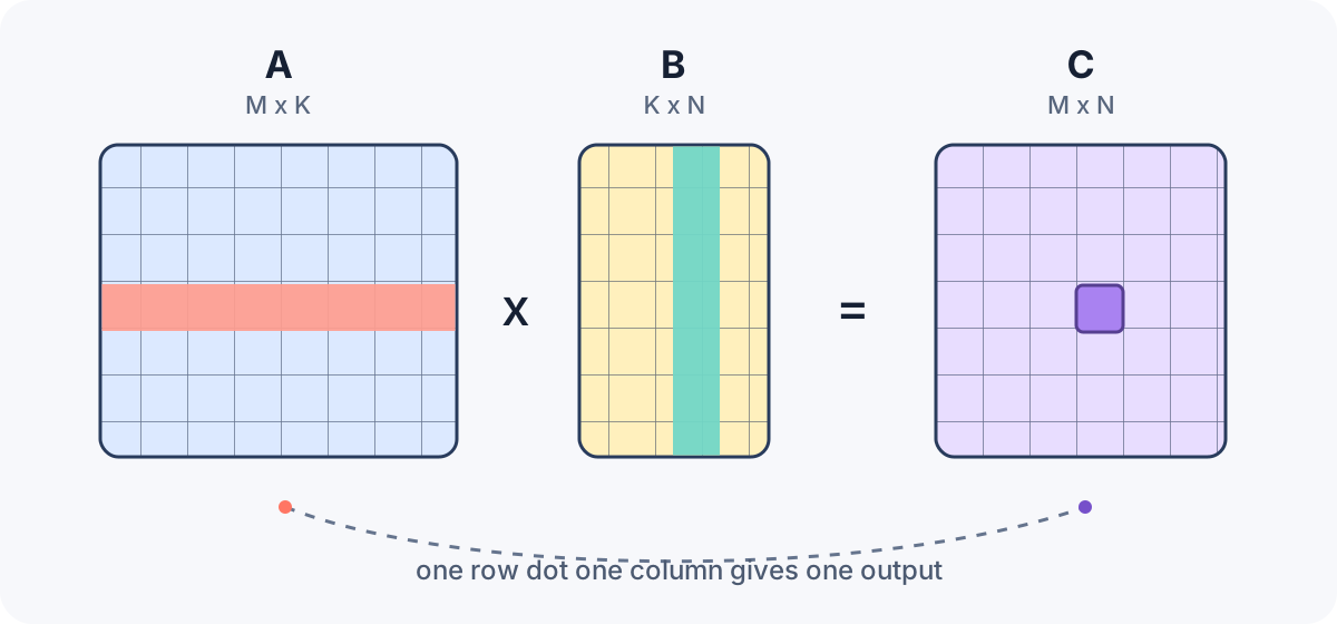

An M by K matrix A multiplied by a K by N matrix B to produce an M by N matrix C. One row of A and one column of B are highlighted because their dot product produces one highlighted output element.

Alright, so let’s get started. The most direct CUDA kernel assigns one thread to every element of $\mathbf{C}$. Each thread walks over the $K$ dimension, computes one dot product, and writes one value to $\mathbf{C}$.

row    <- block_y * block_height + thread_x
column <- block_x * block_width  + thread_y

if row or column is outside C:
    stop

sum <- 0

for inner from 0 to K - 1:
    sum <- sum + A[row, inner] * B[inner, column]

C[row, column] <- sum

Let’s see how efficient this direct kernel is. One thread calculates a dot product of length $K$. That is $K$ multiplications and $K-1$ additions:

\[2K-1 \quad \text{FLOPs}.\]

Across all $MN$ threads, the computation is

\[MN(2K-1)=2MNK-MN \quad \text{FLOPs}.\]

Now count the memory requests. Every thread reads $K$ values from $\mathbf{A}$, reads $K$ values from $\mathbf{B}$, and writes one result to $\mathbf{C}$.

Operation	Elements requested	Bytes requested
Read $\mathbf{A}$	$MNK$	$4MNK$
Read $\mathbf{B}$	$MNK$	$4MNK$
Write $\mathbf{C}$	$MN$	$4MN$
Total	$2MNK+MN$	$4(2MNK+MN)$

Ignoring the cache for a moment, its arithmetic intensity is

\[\begin{aligned} AI_{\text{naive}} &=\frac{2MNK-MN}{4(2MNK+MN)}\\ &=\frac{2K-1}{4(2K+1)}\\ &\approx0.25 \quad \text{FLOPs/byte}. \end{aligned}\]

This means that our implementation is memory bound. But just like GEMV, this number assumes that when a thread asks for one 4-byte float, only those 4 bytes travel through memory. Global-memory transactions do not work like that. The GPU fetches aligned chunks, and any unused bytes in those chunks are wasted.

So before optimizing anything, let us calculate how efficiently our warp uses those transactions. Go back to the first two lines of the pseudocode:

row    <- block_y * block_width  + thread_x
column <- block_x * block_height + thread_y

We made thread_x choose the row and thread_y choose the column.

CUDA places threads into a warp by changing thread_x first. So while thread_y stays fixed, the neighboring threads keep the same column and move across different rows:

thread 0 owns C[row + 0, column]
thread 1 owns C[row + 1, column]
thread 2 owns C[row + 2, column]
...

At one value of inner, those threads read

thread 0 -> A[row + 0, inner]  B[inner, column]
thread 1 -> A[row + 1, inner]  B[inner, column]
thread 2 -> A[row + 2, inner]  B[inner, column]
...

The $\mathbf{B}$ access is fine because every thread asks for the same value. But neighboring threads read $\mathbf{A}$ values that are $K$ elements apart, and later write $\mathbf{C}$ values that are $N$ elements apart.

Using the same simplified 32-byte-sector model as the GEMV chapter, the warp asks for 32 useful FP32 values from $\mathbf{A}$:

\[32\times4=128 \quad \text{useful bytes}.\]

But because those values are far apart, each thread can require a separate 32-byte sector. The warp may therefore transfer

\[32\times32=1024 \quad \text{bytes}.\]

The transaction efficiency of the $\mathbf{A}$ read is only

\[\eta_A =\frac{128}{1024} =\frac{1}{8} =12.5\%.\]

The final $\mathbf{C}$ write has the same efficiency because those 32 output values are also separated by a complete row. The $\mathbf{B}$ read is the one part that behaves well: every thread requests the same value, so one memory transaction can be broadcast across the warp.

So $0.25$ FLOPs/byte was already low, and the strided $\mathbf{A}$ reads and $\mathbf{C}$ writes make the effective traffic even worse. That is now our first target. We will keep one output element per thread, but arrange those elements so neighboring threads work on neighboring columns of the same row.

Let us make threadIdx.x choose the column coordinate instead. Each thread still calculates one output element, but the elements assigned to one warp now lie next to each other in row $r$:

thread 0 -> C[r, column + 0]
thread 1 -> C[r, column + 1]
thread 2 -> C[r, column + 2]
...
thread 31 -> C[r, column + 31]

Let’s use four threads before jumping into the complete warp. During the first loop iteration, the threads read

thread 0 -> A[r, 0]  B[0, column + 0]
thread 1 -> A[r, 0]  B[0, column + 1]
thread 2 -> A[r, 0]  B[0, column + 2]
thread 3 -> A[r, 0]  B[0, column + 3]

During the next iteration, every thread moves to the next row of $\mathbf{B}$:

thread 0 -> A[r, 1]  B[1, column + 0]
thread 1 -> A[r, 1]  B[1, column + 1]
thread 2 -> A[r, 1]  B[1, column + 2]
thread 3 -> A[r, 1]  B[1, column + 3]

If you notice, one thread jumps by $N$ elements through $\mathbf{B}$ over time, but neighboring threads read neighboring values at the same instant. The value from $\mathbf{A}$ is common to all of them, so it can be broadcast across the warp. The final writes to $\mathbf{C}$ are neighboring values too.

For a real warp, the first iteration reads 32 consecutive values from one row of $\mathbf{B}$, the second iteration reads 32 consecutive values from the next row, and so on. Every iteration therefore produces one coalesced chunk.

Great, this is the access pattern we were looking for. The pseudocode now becomes:

column <- block_x * block_width  + thread_x
row    <- block_y * block_height + thread_y

if row or column is outside C:
    stop

sum <- 0

for inner from 0 to K - 1:
    sum <- sum + A[row, inner] * B[inner, column]

C[row, column] <- sum

All we did was change the thread mapping. The math is identical, but the memory access is much better.

Cost after coalescing

The logical work did not change. Every thread still reads $K$ values from $\mathbf{A}$, reads $K$ values from $\mathbf{B}$, and writes one result. So the requested traffic is still $4(2MNK+MN)$ bytes and the arithmetic intensity is still

\[AI_{\text{coalesced}} =AI_{\text{naive}} \approx0.25 \quad \text{FLOPs/byte}.\]

But now we can compare the actual transactions. Under our simplified 32-byte-sector model, one warp behaves like this:

Warp operation	Before remapping	After remapping
Read $\mathbf{A}$ at one `inner`	32 separated sectors = 1024 bytes	1 broadcast sector = 32 bytes
Read $\mathbf{B}$ at one `inner`	1 broadcast sector = 32 bytes	4 consecutive sectors = 128 bytes
Write 32 values to $\mathbf{C}$	32 separated sectors = 1024 bytes	4 consecutive sectors = 128 bytes

For one step of the dot product, the input traffic falls from

\[1024+32=1056 \quad \text{bytes}\]

\[32+128=160 \quad \text{bytes}.\]

The output transaction is eight times smaller too. This does not mean that the kernel must become exactly that much faster. The requested-byte arithmetic intensity did not change. What changed is that the same requests are now served with much cleaner transactions.

But there is still a deeper problem hiding inside the requested traffic itself. Take $\mathbf{A}$ first. The matrix contains only $MK$ values, but our kernel requests $MNK$ values from it. Why? Because every output column repeats the same row of $\mathbf{A}$.

The same thing happens to $\mathbf{B}$. It contains only $KN$ values, but our kernel requests $MNK$ values from it because every output row repeats the same column of $\mathbf{B}$.

So coalescing fixed how the requests reach memory. It did not fix how many times we make those requests.

Now the next question is much more specific: instead of letting each thread ask for its own copy, can a block load a small group of $\mathbf{A}$ and $\mathbf{B}$ values once, put them somewhere nearby, and reuse them for several outputs?

That nearby place is shared memory.

Shared memory tiling

Until now, every thread has behaved like it is alone. It loads the values it needs, computes one output, and writes the answer.

Shared memory changes the unit of cooperation. Instead of thinking “one thread computes one dot product from global memory,” we think:

one block owns one small rectangle of C
the block loads the matching small rectangles of A and B
all threads reuse those loaded values

That small rectangle is a tile. Tiling is not a different matrix multiplication algorithm. It is the same dot products, but grouped so nearby threads can share nearby data.

There are three tiles to keep separate:

Tile	Where it lives	What it means
Output tile	Registers, then $\mathbf{C}$	The fixed rectangle of $\mathbf{C}$ owned by one block
$\mathbf{A}$ input tile	Shared memory	The next slice of the needed rows of $\mathbf{A}$
$\mathbf{B}$ input tile	Shared memory	The next slice of the needed columns of $\mathbf{B}$

Inside that block, each thread can still own one output element. The difference is that the inputs are no longer loaded separately by every thread. The block loads a small piece of $\mathbf{A}$ and a small piece of $\mathbf{B}$ once, puts them in shared memory, and then all threads reuse those values.

Suppose the block owns a $T\times T$ tile of $\mathbf{C}$. Those $T^2$ outputs use the same $T$ rows of $\mathbf{A}$ and the same $T$ columns of $\mathbf{B}$. But each dot product still runs across the full $K$ dimension. So we do not try to load the full rows and columns at once. We walk across $K$ in chunks:

load the next T columns from the needed rows of A
load the next T rows from the needed columns of B
synchronize
use those two input tiles to add a partial result to the fixed C tile
synchronize
move to the next K tile

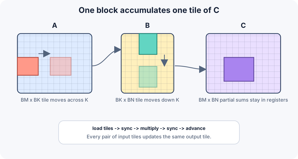
This is the key picture: the output tile does not move. The $\mathbf{A}$ and $\mathbf{B}$ input tiles move along $K$, and every pair contributes one more piece to the same output accumulators.

A small example

Let’s use a $4\times4$ multiplication and a tile size of 2. We want the top-left $2\times2$ tile of $\mathbf{C}$:

\[\begin{bmatrix} C_{00}&C_{01}\\ C_{10}&C_{11} \end{bmatrix}.\]

Every one of these four outputs is a dot product of length 4. With a tile size of 2, the block cannot finish the dot products from one pair of input tiles. It computes the first two terms, keeps the partial sums, then loads the next two terms.

First, take the $k=0,1$ part:

\[\mathbf{A}^{(0)}= \begin{bmatrix} a_{00}&a_{01}\\ a_{10}&a_{11} \end{bmatrix}, \qquad \mathbf{B}^{(0)}= \begin{bmatrix} b_{00}&b_{01}\\ b_{10}&b_{11} \end{bmatrix}.\]

Multiplying these two small tiles gives only the first half of each dot product:

\[\mathbf{C}_{0:2,0:2} \mathrel{+}=\mathbf{A}^{(0)}\mathbf{B}^{(0)}.\]

For example, the partial value of $C_{00}$ now contains

\[a_{00}b_{00}+a_{01}b_{10}.\]

That is not enough. The full dot product also needs the $k=2,3$ terms. So the block moves forward along $K$ and loads

\[\mathbf{A}^{(1)}= \begin{bmatrix} a_{02}&a_{03}\\ a_{12}&a_{13} \end{bmatrix}, \qquad \mathbf{B}^{(1)}= \begin{bmatrix} b_{20}&b_{21}\\ b_{30}&b_{31} \end{bmatrix}.\]

These are multiplied and added to the same output tile:

\[\mathbf{C}_{0:2,0:2} \mathrel{+}=\mathbf{A}^{(1)}\mathbf{B}^{(1)}.\]

Now $C_{00}$ contains

\[a_{00}b_{00} +a_{01}b_{10} +a_{02}b_{20} +a_{03}b_{30},\]

which is the complete dot product. The other three outputs in the tile are completed in the same way.

So tiling is not “multiply random small matrices and stitch the answers together later.” Each block owns one fixed tile of $\mathbf{C}$. The $\mathbf{A}$ and $\mathbf{B}$ tiles are just consecutive $K$-slices needed by the dot products for that same output tile.

Turning the idea into code

We said that one block owns a $T\times T$ tile of $\mathbf{C}$. For our first tiled implementation, let us give that block $T\times T$ threads as well. Thread $(t_y,t_x)$ owns the output at local position $(t_y,t_x)$ inside the tile.

Each input tile also contains $T^2$ values. Since the block has $T^2$ threads, the loading work divides naturally: every thread copies one value from $\mathbf{A}$ and one value from $\mathbf{B}$ into shared memory. After the complete tiles have arrived, that thread uses one row of the shared $\mathbf{A}$ tile and one column of the shared $\mathbf{B}$ tile to update its output.

Here is the same loop visually. Watch what stays fixed and what changes. The $\mathbf{C}$ tile stays fixed. The shared $\mathbf{A}$ and $\mathbf{B}$ tiles are reused for one chunk of $K$, then overwritten with the next chunk only after every thread is done reading them.

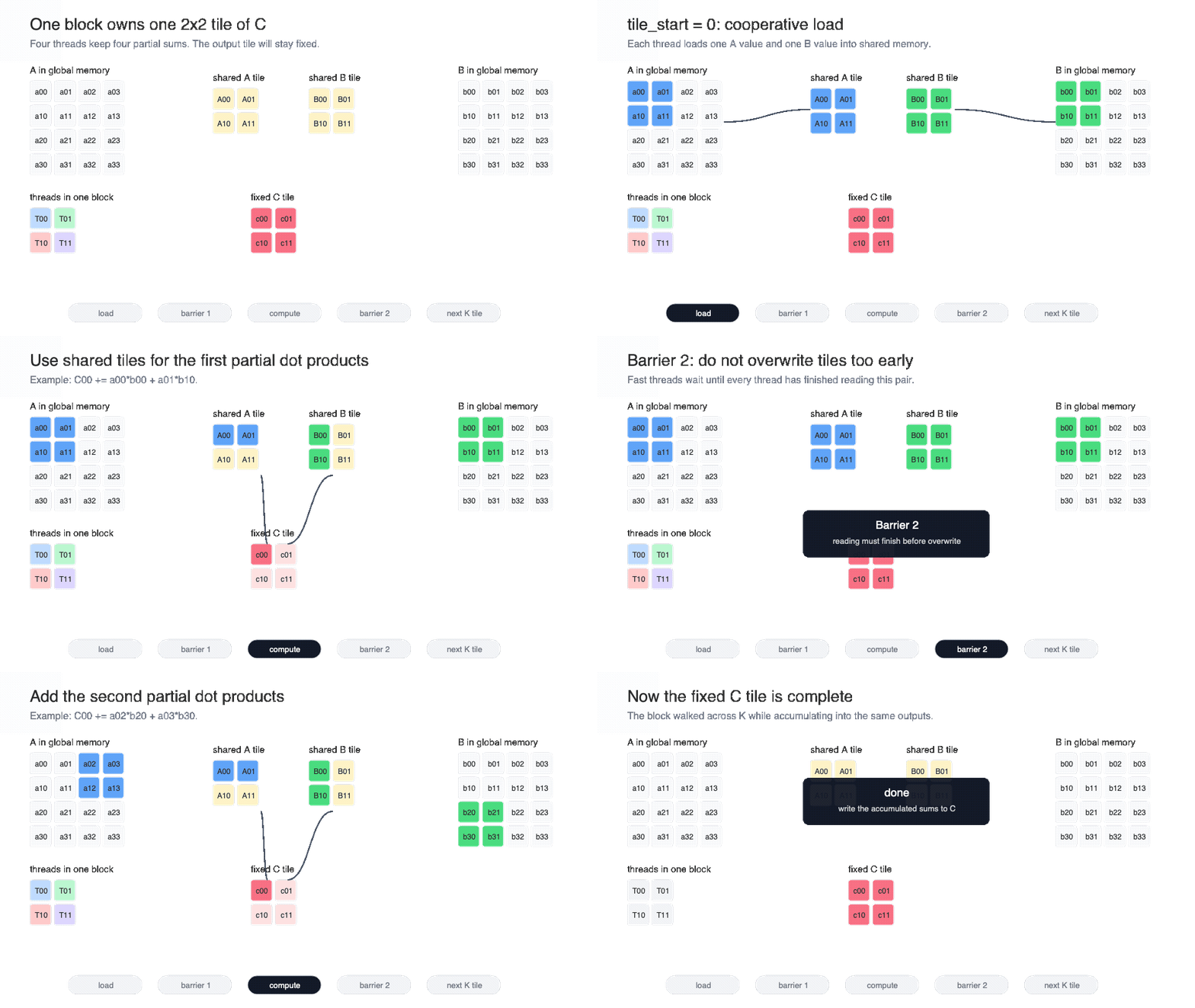
Animation of shared-memory tiled GEMM. A block owns one fixed tile of C, cooperatively loads A and B tiles into shared memory, waits at the first barrier, computes partial dot products, waits at the second barrier, then overwrites shared memory with the next K tile.

The complete schedule is:

create a shared tile for A
create a shared tile for B

row, column <- the output element owned by this thread
sum <- 0

for tile_start from 0 to K - 1 in steps of tile_size:
    each thread loads one A value into the shared A tile
    each thread loads one B value into the shared B tile
    use zero when a value falls outside the matrix

    wait until both tiles are complete

    for inner from 0 to tile_size - 1:
        sum <- sum + A_tile[local_row, inner]
                   * B_tile[inner, local_column]

    wait until every thread has finished using the tiles

if row and column are inside C:
    C[row, column] <- sum

Why do we need two barriers?

The tile is loaded cooperatively. Every thread contributes only one value, but the dot product performed by one thread reads values loaded by many other threads. Without the first barrier, a fast thread could begin its dot product while some entries of the shared tiles have not been written yet. It would then multiply incomplete or stale data.

The second barrier protects the same shared-memory arrays from being reused too early. After finishing its own dot product, a fast thread may move to the next iteration and start loading the next pair of tiles. A slower thread may still be reading the current pair. Without a barrier between those two actions, the fast thread could overwrite a value that the slower thread has not used yet.

So the first barrier separates loading from reading, and the second separates reading the current tiles from overwriting them with the next tiles.

Also notice the zeroes for out-of-bounds values. We cannot just return from the kernel when one thread falls outside the matrix because the other threads will eventually wait for it at __syncthreads(). Instead, edge threads load zero and still participate in the barriers.

Cost after tiling

Let’s count the same $4\times4$ example with tile size 2.

During the first chunk of $K$, the block loads this much data into shared memory:

Tile	Values loaded
$\mathbf{A}^{(0)}$	$2\times2=4$
$\mathbf{B}^{(0)}$	$2\times2=4$
Total	8 values

These 8 values update the four outputs in the fixed $\mathbf{C}$ tile:

\[\begin{bmatrix} C_{00}&C_{01}\\ C_{10}&C_{11} \end{bmatrix}.\]

Each output gets two updates from this chunk. For example,

\[C_{00} \mathrel{+}=a_{00}b_{00} +a_{01}b_{10}.\]

In CUDA, this update usually becomes a fused multiply-add, or FMA:

sum <- sum + a * b

One FMA is one instruction, but it represents two floating-point operations: one multiply and one add.

So for this one chunk, the block performs

\[4 \text{ outputs}\times2 \text{ FMAs per output} =8 \text{ FMAs}.\]

That is

\[8\times2=16 \quad \text{FLOPs}.\]

The global-memory traffic for the chunk is

\[8 \text{ FP32 values}\times4 =32 \quad \text{bytes}.\]

So the arithmetic intensity for this tiled chunk is

\[\frac{16}{32} =0.5 \quad \text{FLOPs/byte}.\]

That is already twice the requested-byte intensity of the direct kernel. The reason is not that we changed the math. The reason is that the 8 values loaded into shared memory were reused across four outputs.

Now generalize the same count to a $T\times T$ tile.

For one chunk of $K$, the block loads

\[T^2+T^2=2T^2\]

values from global memory. Those values update $T^2$ outputs. Each output gets $T$ fused multiply-adds from this chunk, so the block performs

\[T^3 \quad \text{FMAs}.\]

Since one FMA counts as two FLOPs, the arithmetic intensity at the global-memory boundary is

\[\begin{aligned} AI_{\text{tile}} &=\frac{2T^3}{4(2T^2)}\\ &=\frac{T}{4} \quad \text{FLOPs/byte}. \end{aligned}\]

The intensity now grows with $T$. Bigger output tiles create more reuse because the same input values feed more outputs. This time the improvement did not come from changing how a warp groups its requests. It came from making one global-memory load feed many multiply-adds.

We have now fixed global-memory reuse. But if we inspect the inner loop, there is another problem waiting for us.

One output per thread is not enough

Shared memory fixed the global-memory problem. The block now loads a tile once and reuses it across many output elements.

Sounds neat and perfect right?

Except we should do the same thing we did in GEMV: freeze the kernel and look at what is happening at one instant.

This time, instead of freezing a warp, freeze one thread.

Say a thread owns only one output:

result -> C[row, column]

At one value of inner, it does this:

A_value <- A_tile[row, inner]
B_value <- B_tile[inner, column]

result <- result + A_value * B_value

So for one multiply-add, the thread performs two shared-memory loads. One load comes from the shared $\mathbf{A}$ tile, and one load comes from the shared $\mathbf{B}$ tile.

Now look at the output right below it:

C[row + 0, column] uses B_tile[inner, column]
C[row + 1, column] uses B_tile[inner, column]
C[row + 2, column] uses B_tile[inner, column]
...

All of these outputs need the same $\mathbf{B}$ value at this value of inner. But in our current kernel, they belong to different threads. Each thread loads that same $\mathbf{B}$ value from shared memory, uses it once, and moves on.

See the problem? Shared memory made the value closer, but it did not make the thread reuse it. The reuse exists between neighboring outputs, while each thread owns only one output.

What if one thread owned two outputs from the same column?

result0 -> C[row + 0, column]
result1 -> C[row + 1, column]

Now at the same inner, the thread can do

B_value <- B_tile[inner, column]

result0 <- result0 + A_tile[row + 0, inner] * B_value
result1 <- result1 + A_tile[row + 1, inner] * B_value

Now one shared-memory load from $\mathbf{B}$ produces two multiply-adds. The two partial sums live in registers, so the thread can keep both of them around while it walks through the loop.

That is the next target. The block still owns a larger output tile, but each thread now owns a smaller tile inside it. This smaller per-thread tile is often called a micro-tile, and its partial sums live in registers.

1D register tiling

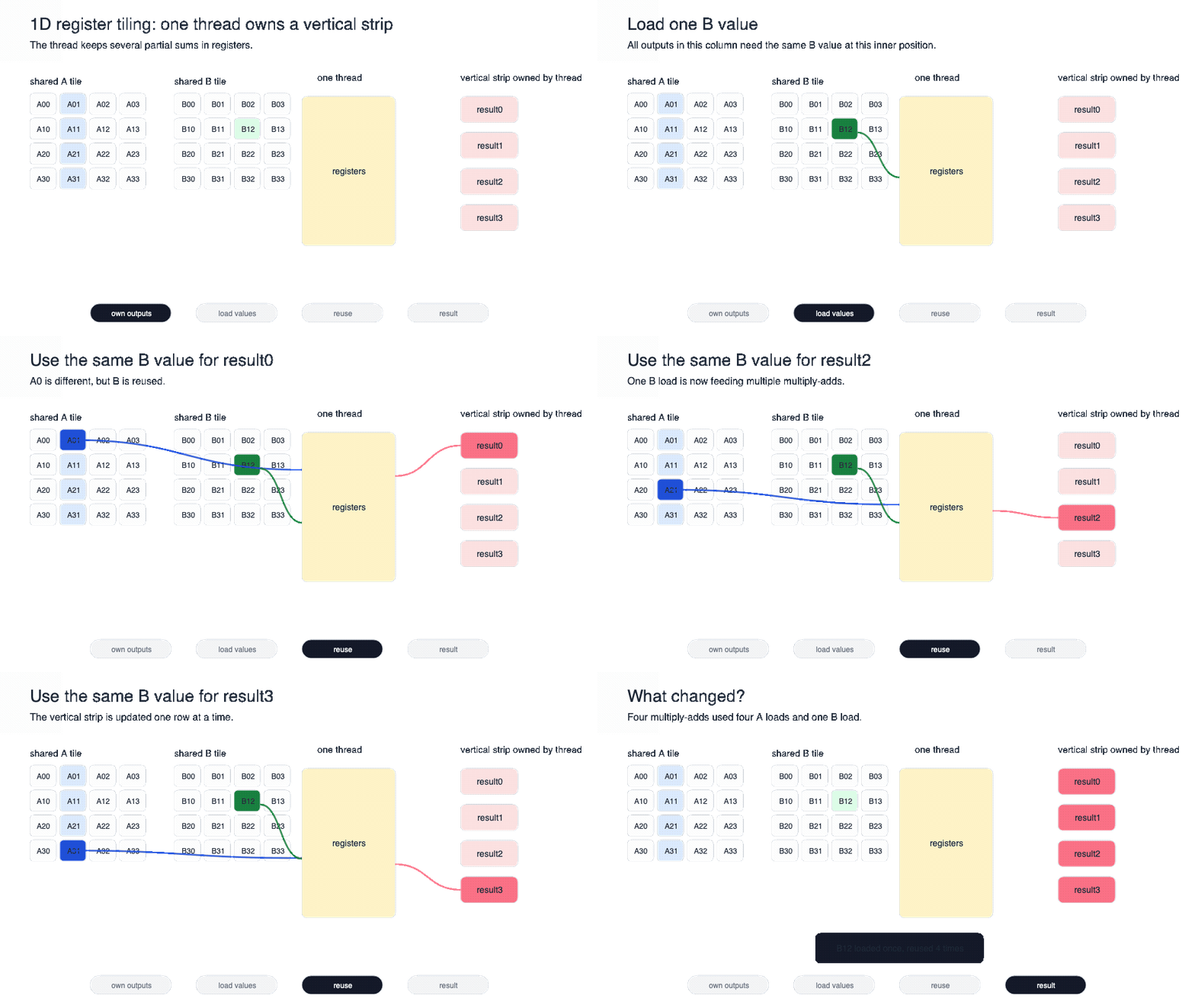
Start with the smallest useful change. Instead of giving a thread one output, give it a vertical strip of outputs:

result0 -> C[row + 0, column]
result1 -> C[row + 1, column]
result2 -> C[row + 2, column]
...

Let us use four outputs for the example. At one value of inner, all four outputs need the same $\mathbf{B}$ value:

B_value <- B_tile[inner, thread_column]

result0 <- result0 + A_tile[row + 0, inner] * B_value
result1 <- result1 + A_tile[row + 1, inner] * B_value
result2 <- result2 + A_tile[row + 2, inner] * B_value
result3 <- result3 + A_tile[row + 3, inner] * B_value

The thread still loads four different $\mathbf{A}$ values, because the four outputs come from four different rows. But it loads the $\mathbf{B}$ value once and reuses it four times.

This is one-dimensional register tiling. One dimension of the block’s output tile now lives inside a single thread.

Here is the same idea visually. Watch the $\mathbf{B}$ value: it is loaded once and then reused across the vertical strip of outputs owned by the thread.

Animation of one-dimensional register tiling. One thread owns a vertical strip of outputs, loads one B value, and reuses it across several multiply-adds with different A values.

Cost of 1D register tiling

In the four-output example, the thread performs four multiply-adds.

The old tiled kernel would need two shared-memory loads per multiply-add:

4 multiply-adds -> 8 shared-memory loads

With the vertical strip, the thread loads four $\mathbf{A}$ values and one $\mathbf{B}$ value:

4 multiply-adds -> 5 shared-memory loads

So we did not change the math. We changed which outputs one thread owns, and that let one $\mathbf{B}$ load feed several multiply-adds.

If the thread owns $T_M$ outputs in the same column, then one inner-loop step uses

\[T_M + 1\]

shared-memory loads to produce

\[T_M\]

multiply-adds. The bigger $T_M$ gets, the more useful work we get out of the one $\mathbf{B}$ value loaded into a register.

But notice the asymmetry. We reused $\mathbf{B}$. We did not reuse $\mathbf{A}$. Each $\mathbf{A}$ value still updates exactly one result inside the thread.

Can we reuse both?

2D register tiling

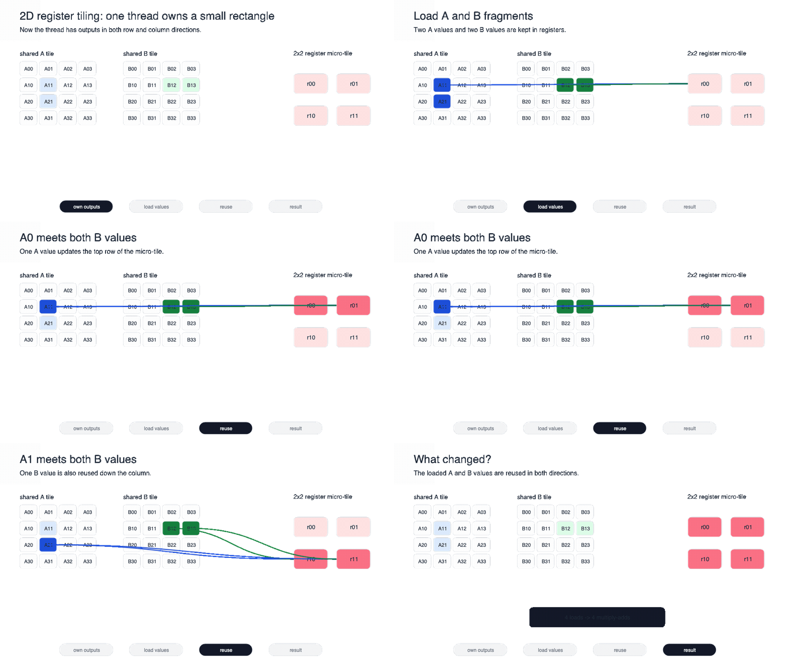
To reuse both sides, the thread needs outputs in both directions.

Instead of a vertical strip, give one thread a small rectangle of $\mathbf{C}$:

result00 -> C[row + 0, column + 0]
result01 -> C[row + 0, column + 1]
result10 -> C[row + 1, column + 0]
result11 -> C[row + 1, column + 1]

This little rectangle is the thread’s register micro-tile. The partial sums are stored in registers until the final write to $\mathbf{C}$.

Now freeze the thread at one value of inner.

It loads two values from the shared $\mathbf{A}$ tile:

A0 <- A_tile[row + 0, inner]
A1 <- A_tile[row + 1, inner]

and two values from the shared $\mathbf{B}$ tile:

B0 <- B_tile[inner, column + 0]
B1 <- B_tile[inner, column + 1]

Now every $\mathbf{A}$ value can meet every $\mathbf{B}$ value:

result00 <- result00 + A0 * B0
result01 <- result01 + A0 * B1
result10 <- result10 + A1 * B0
result11 <- result11 + A1 * B1

That is the entire trick. We loaded four shared-memory values and produced four multiply-adds. More importantly, each loaded value was used twice.

This is a tiny outer product inside one thread. A column of $\mathbf{A}$ values meets a row of $\mathbf{B}$ values, and together they update a small rectangle of $\mathbf{C}$.

The animation below shows that crossing more directly. The $\mathbf{A}$ values move down the rows, the $\mathbf{B}$ values move across the columns, and the thread updates the whole $2\times2$ register micro-tile.

Animation of two-dimensional register tiling. One thread owns a 2 by 2 register micro-tile, loads two A values and two B values, and reuses them in both directions to update four outputs.

For a general $T_M\times T_N$ micro-tile, the inner loop looks like this:

for inner from 0 to BK - 1:
    load TM values from A_tile into registers
    load TN values from B_tile into registers

    for each A value:
        for each B value:
            update one result register

Every $\mathbf{A}$ value is reused across $T_N$ columns. Every $\mathbf{B}$ value is reused across $T_M$ rows.

Cost of 2D register tiling

Stay with the $2\times2$ micro-tile for one more second.

The thread loaded

\[2+2=4\]

shared-memory values and performed

\[2\times2=4\]

multiply-adds.

For a larger $8\times8$ micro-tile, the same idea gives

\[8+8=16 \quad \text{shared-memory loads},\] \[8\times8=64 \quad \text{multiply-adds}.\]

Compare that with the first shared-memory tiled kernel. There, 16 shared-memory loads would only produce 8 multiply-adds, because every multiply-add loaded one $\mathbf{A}$ value and one $\mathbf{B}$ value.

Here, the same 16 loads produce 64 multiply-adds because the values are reused inside the thread.

That is why register tiling matters. Shared memory made global loads reusable across the block. Registers make shared-memory loads reusable inside one thread.

Choosing the tile sizes

So we can just keep making the thread tile larger and reuse even more? In reality, no, because registers are limited.

Every output owned by a thread needs one accumulator register. A $2\times2$ micro-tile needs 4 accumulators. An $8\times8$ micro-tile needs

\[8\times8=64\]

accumulator registers, before counting loop variables, addresses, and the temporary $\mathbf{A}$ and $\mathbf{B}$ fragments.

So tile size is a tradeoff.

Larger micro-tiles reuse shared-memory values more aggressively, but they also increase register pressure. If a thread uses too many registers, fewer warps can live on the SM at the same time. If the pressure gets really high, the compiler may spill values to local memory, which is exactly what we were trying to avoid.

The final kernel uses

\[B_M=B_N=128, \qquad B_K=8, \qquad T_M=T_N=8.\]

That means one block owns a $128\times128$ tile of $\mathbf{C}$, and each thread owns an $8\times8$ micro-tile inside it. So the block needs

\[\frac{128}{8}\times\frac{128}{8} =16\times16 =256\]

threads.

For one 8-wide step along $K$, the block loads

\[128\times8+8\times128=2048\]

FP32 values into shared memory. Those values update the same $128\times128$ output tile for 8 positions of the inner dimension.

Do enough reuse to make shared-memory loads worthwhile, but not so much per-thread state that the kernel collapses under register pressure.

Final kernel

Now we can put the pieces together. But pasting the complete CUDA kernel here would interrupt the flow more than it would help.

At this point, the final implementation is just the ideas above combined in one place:

one block owns a BM x BN output tile
one thread owns a TM x TN micro-tile
for each BK chunk along K:
    load A and B tiles into shared memory
    synchronize
    update the register micro-tile
    synchronize
write the register results back to C

The complete CUDA source, including the launcher, lives here:

kernels/gemm/05_2d_register_tiled_kernel.cu

A few things are worth looking for when you open that file:

A_tile and B_tile are the shared-memory tiles.
results is the per-thread register micro-tile.
the two __syncthreads() calls are the same two barriers we discussed earlier.
the inner loop loads short $\mathbf{A}$ and $\mathbf{B}$ fragments into registers and updates the thread’s micro-tile.

Comparing the kernels

Let’s put the complete progression together:

Kernel	Outputs per thread	What changed	What still costs us
Naive row-first	1	Direct implementation	Strided $\mathbf{A}$ loads and $\mathbf{C}$ stores
Coalesced direct	1	x-lanes own consecutive columns	Inputs are still requested for every output
Shared-memory tiled	1	One global load feeds many threads	Two shared-memory loads per multiply-add
1D register tiled	$T_M$	Reuses one $\mathbf{B}$ value	Reuse is only in one direction
2D register tiled	$T_MT_N$	Reuses both input fragments	Register pressure

Notice how every optimization moves the bottleneck one level closer to the compute units.

First, global-memory access was bad. We fixed coalescing.

Then, global-memory access was repeated. We added shared-memory tiles.

Then, shared-memory values were used only once per thread. We added register micro-tiles.

Another way to read the whole chapter is:

coalescing:       make neighboring threads request neighboring memory
shared tiling:    make one global load serve many threads
register tiling:  make one shared-memory load serve many outputs in one thread

I am deliberately not putting performance numbers in this table yet. A number without a GPU model, matrix shape, CUDA version, warm-up, and timing method is not useful. These kernels need to be benchmarked against the same reference on the same machine. We should also inspect register usage and spills, because a kernel with more reuse on paper can still lose if the compiler runs out of registers.

Main takeaways

GEMM has a lot of arithmetic intensity only when we actually reuse the inputs. The equation gives us the opportunity. The kernel has to make that reuse happen.
Thread mapping matters before tiling even begins. Since threadIdx.x changes fastest inside a warp, mapping it to output columns gives us consecutive $\mathbf{B}$ reads and $\mathbf{C}$ writes.
Coalescing and reuse are different things. Coalescing makes one warp request memory efficiently. Tiling removes repeated global-memory requests by keeping input values in shared memory.
A block owns one fixed output tile. It walks along the $K$ dimension, loading pairs of input tiles and accumulating partial dot products into the same output values.
Shared-memory tiling is only the first level of reuse. If every thread computes one output, it still loads two shared values for every multiply-add.
Register tiling gives one thread multiple outputs. A 2D micro-tile lets the thread load short fragments from $\mathbf{A}$ and $\mathbf{B}$ and form an outer product, reusing both fragments many times.
Bigger tiles are not automatically better. Shared-memory capacity, register pressure, occupancy, edge waste, and matrix shape all affect the result.

The GEMM equation never changed. What changed was ownership. First one thread owned one output. Then one block owned an output tile. Finally, every thread owned a micro-tile inside that block and kept its partial results in registers.

That is the main lesson. A fast GEMM kernel is still just the same collection of dot products. The hard part is deciding how long each value stays close to the processors, and how many times we can use it before loading something new.

Citation

For attribution in academic contexts, please cite this work as:

    Mishra, Anshuman. "How to make your models fast." Online, 2026.

or as a BibTeX entry:

    @book{how-to-make-your-models-fast,
      title = {How to make your models fast},
      author = {Mishra, Anshuman},
      howpublished = {Online},
      url = {https://athleticcoder21.github.io/inference-book/},
      year = {2026}
    }